Optional Lab: Gradient Descent for Logistic Regression

Goals

In this lab, you will:

• update gradient descent for logistic regression.
• explore gradient descent on a familiar data set

import copy, math
import numpy as np
%matplotlib widget
import matplotlib.pyplot as plt
from lab_utils_common import  dlc, plot_data, plt_tumor_data, sigmoid, compute_cost_logistic
from plt_quad_logistic import plt_quad_logistic, plt_prob
plt.style.use('./deeplearning.mplstyle')

Data set

Let's start with the same two feature data set used in the decision boundary lab.

X_train = np.array([[0.5, 1.5], [1,1], [1.5, 0.5], [3, 0.5], [2, 2], [1, 2.5]])
y_train = np.array([0, 0, 0, 1, 1, 1])

As before, we'll use a helper function to plot this data. The data points with label $y=1$ are shown as red crosses, while the data points with label $y=0$ are shown as blue circles.

fig,ax = plt.subplots(1,1,figsize=(4,4))
plot_data(X_train, y_train, ax)

ax.axis([0, 4, 0, 3.5])
ax.set_ylabel('$x_1$', fontsize=12)
ax.set_xlabel('$x_0$', fontsize=12)
plt.show()

Logistic Gradient Descent

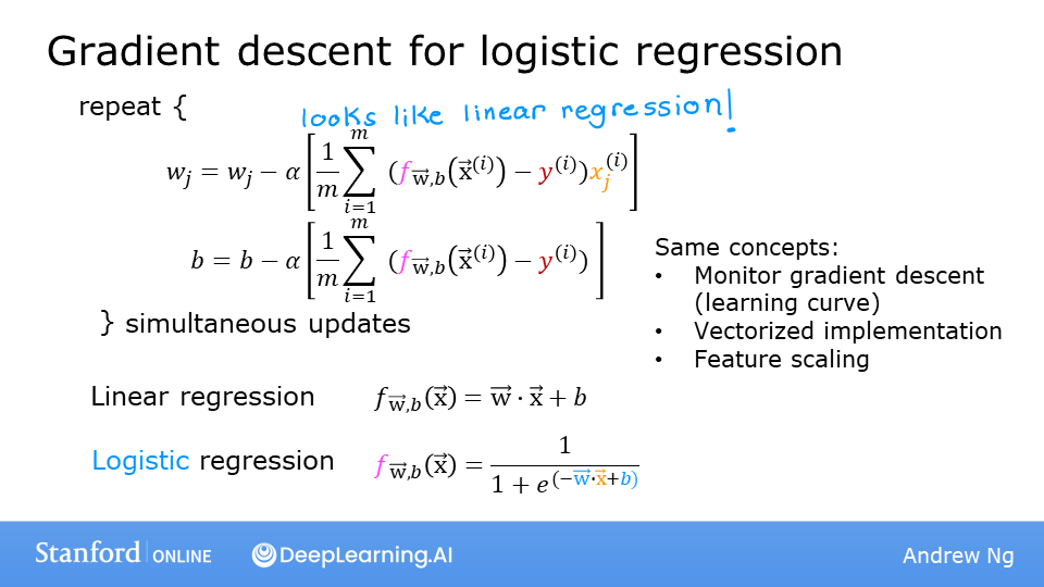
Recall the gradient descent algorithm utilizes the gradient calculation: $$\begin{align*} &\text{repeat until convergence:} \; \lbrace \\ & \; \; \;w_j = w_j - \alpha \frac{\partial J(\mathbf{w},b)}{\partial w_j} \tag{1} \; & \text{for j := 0..n-1} \\ & \; \; \; \; \;b = b - \alpha \frac{\partial J(\mathbf{w},b)}{\partial b} \\ &\rbrace \end{align*}$$

Where each iteration performs simultaneous updates on $w_j$ for all $j$, where $$\begin{align*} \frac{\partial J(\mathbf{w},b)}{\partial w_j} &= \frac{1}{m} \sum\limits_{i = 0}^{m-1} (f_{\mathbf{w},b}(\mathbf{x}^{(i)}) - y^{(i)})x_{j}^{(i)} \tag{2} \\ \frac{\partial J(\mathbf{w},b)}{\partial b} &= \frac{1}{m} \sum\limits_{i = 0}^{m-1} (f_{\mathbf{w},b}(\mathbf{x}^{(i)}) - y^{(i)}) \tag{3} \end{align*}$$

• m is the number of training examples in the data set
• $f_{\mathbf{w},b}(x^{(i)})$ is the model's prediction, while $y^{(i)}$ is the target
• For a logistic regression model
  $z = \mathbf{w} \cdot \mathbf{x} + b$
  $f_{\mathbf{w},b}(x) = g(z)$
  where $g(z)$ is the sigmoid function:
  $g(z) = \frac{1}{1+e^{-z}}$

Gradient Descent Implementation

The gradient descent algorithm implementation has two components:

• The loop implementing equation (1) above. This is gradient_descent below and is generally provided to you in optional and practice labs.
• The calculation of the current gradient, equations (2,3) above. This is compute_gradient_logistic below. You will be asked to implement this week's practice lab.

Calculating the Gradient, Code Description

Implements equation (2),(3) above for all $w_j$ and $b$. There are many ways to implement this. Outlined below is this:

• initialize variables to accumulate dj_dw and dj_db

• for each example

  • calculate the error for that example $g(\mathbf{w} \cdot \mathbf{x}^{(i)} + b) - \mathbf{y}^{(i)}$
  • for each input value $x_{j}^{(i)}$ in this example,
    • multiply the error by the input $x_{j}^{(i)}$, and add to the corresponding element of dj_dw. (equation 2 above)
  • add the error to dj_db (equation 3 above)

• divide dj_db and dj_dw by total number of examples (m)

• note that $\mathbf{x}^{(i)}$ in numpy X[i,:] or X[i] and $x_{j}^{(i)}$ is X[i,j]

def compute_gradient_logistic(X, y, w, b): 
    """
    Computes the gradient for linear regression 
 
    Args:
      X (ndarray (m,n): Data, m examples with n features
      y (ndarray (m,)): target values
      w (ndarray (n,)): model parameters  
      b (scalar)      : model parameter
    Returns
      dj_dw (ndarray (n,)): The gradient of the cost w.r.t. the parameters w. 
      dj_db (scalar)      : The gradient of the cost w.r.t. the parameter b. 
    """
    m,n = X.shape
    dj_dw = np.zeros((n,))                           #(n,)
    dj_db = 0.

    for i in range(m):
        f_wb_i = sigmoid(np.dot(X[i],w) + b)          #(n,)(n,)=scalar
        err_i  = f_wb_i  - y[i]                       #scalar
        for j in range(n):
            dj_dw[j] = dj_dw[j] + err_i * X[i,j]      #scalar
        dj_db = dj_db + err_i
    dj_dw = dj_dw/m                                   #(n,)
    dj_db = dj_db/m                                   #scalar
        
    return dj_db, dj_dw  

Check the implementation of the gradient function using the cell below.

X_tmp = np.array([[0.5, 1.5], [1,1], [1.5, 0.5], [3, 0.5], [2, 2], [1, 2.5]])
y_tmp = np.array([0, 0, 0, 1, 1, 1])
w_tmp = np.array([2.,3.])
b_tmp = 1.
dj_db_tmp, dj_dw_tmp = compute_gradient_logistic(X_tmp, y_tmp, w_tmp, b_tmp)
print(f"dj_db: {dj_db_tmp}" )
print(f"dj_dw: {dj_dw_tmp.tolist()}" )

Expected output

dj_db: 0.49861806546328574
dj_dw: [0.498333393278696, 0.49883942983996693]

Gradient Descent Code

The code implementing equation (1) above is implemented below. Take a moment to locate and compare the functions in the routine to the equations above.

def gradient_descent(X, y, w_in, b_in, alpha, num_iters): 
    """
    Performs batch gradient descent
    
    Args:
      X (ndarray (m,n)   : Data, m examples with n features
      y (ndarray (m,))   : target values
      w_in (ndarray (n,)): Initial values of model parameters  
      b_in (scalar)      : Initial values of model parameter
      alpha (float)      : Learning rate
      num_iters (scalar) : number of iterations to run gradient descent
      
    Returns:
      w (ndarray (n,))   : Updated values of parameters
      b (scalar)         : Updated value of parameter 
    """
    # An array to store cost J and w's at each iteration primarily for graphing later
    J_history = []
    w = copy.deepcopy(w_in)  #avoid modifying global w within function
    b = b_in
    
    for i in range(num_iters):
        # Calculate the gradient and update the parameters
        dj_db, dj_dw = compute_gradient_logistic(X, y, w, b)   

        # Update Parameters using w, b, alpha and gradient
        w = w - alpha * dj_dw               
        b = b - alpha * dj_db               
      
        # Save cost J at each iteration
        if i<100000:      # prevent resource exhaustion 
            J_history.append( compute_cost_logistic(X, y, w, b) )

        # Print cost every at intervals 10 times or as many iterations if < 10
        if i% math.ceil(num_iters / 10) == 0:
            print(f"Iteration {i:4d}: Cost {J_history[-1]}   ")
        
    return w, b, J_history         #return final w,b and J history for graphing

Let's run gradient descent on our data set.

w_tmp  = np.zeros_like(X_train[0])
b_tmp  = 0.
alph = 0.1
iters = 10000

w_out, b_out, _ = gradient_descent(X_train, y_train, w_tmp, b_tmp, alph, iters) 
print(f"\nupdated parameters: w:{w_out}, b:{b_out}")

Let's plot the results of gradient descent:

fig,ax = plt.subplots(1,1,figsize=(5,4))
# plot the probability 
plt_prob(ax, w_out, b_out)

# Plot the original data
ax.set_ylabel(r'$x_1$')
ax.set_xlabel(r'$x_0$')   
ax.axis([0, 4, 0, 3.5])
plot_data(X_train,y_train,ax)

# Plot the decision boundary
x0 = -b_out/w_out[0]
x1 = -b_out/w_out[1]
ax.plot([0,x0],[x1,0], c=dlc["dlblue"], lw=1)
plt.show()

In the plot above:

• the shading reflects the probability y=1 (result prior to decision boundary)
• the decision boundary is the line at which the probability = 0.5

Another Data set

Let's return to a one-variable data set. With just two parameters, $w$, $b$, it is possible to plot the cost function using a contour plot to get a better idea of what gradient descent is up to.

x_train = np.array([0., 1, 2, 3, 4, 5])
y_train = np.array([0,  0, 0, 1, 1, 1])

As before, we'll use a helper function to plot this data. The data points with label $y=1$ are shown as red crosses, while the data points with label $y=0$ are shown as blue circles.

fig,ax = plt.subplots(1,1,figsize=(4,3))
plt_tumor_data(x_train, y_train, ax)
plt.show()

In the plot below, try:

• changing $w$ and $b$ by clicking within the contour plot on the upper right.
  • changes may take a second or two
  • note the changing value of cost on the upper left plot.
  • note the cost is accumulated by a loss on each example (vertical dotted lines)
• run gradient descent by clicking the orange button.
  • note the steadily decreasing cost (contour and cost plot are in log(cost)
  • clicking in the contour plot will reset the model for a new run
• to reset the plot, rerun the cell

w_range = np.array([-1, 7])
b_range = np.array([1, -14])
quad = plt_quad_logistic( x_train, y_train, w_range, b_range )

Congratulations!

You have:

• examined the formulas and implementation of calculating the gradient for logistic regression
• utilized those routines in
  • exploring a single variable data set
  • exploring a two-variable data set